for full screen
## Import the dataset

osterman <- data_read("https://cgmoreh.github.io/HSS8005/data/osterman_t3.dta")

## Set a seed for being able to reproduce the random sampling in the next step
set.seed(1234)

## Select countries and keep 50 respondents per country at random
osterman <- osterman %>%
  filter(cntry %in% c("GB", "IE", "DE", "FR", "HU", "PL", "PT", "ES")) %>%
group_by(cntry) %>% slice_sample(n=50) %>% ungroup() 
Quantitative analysis
Week 5
Hierarchies
Hierarchical data structures and multilevel modelling
A brief review of single-level regression
A brief review of single-level regression
- We aim to model an outcome measurement, our
estimand
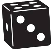
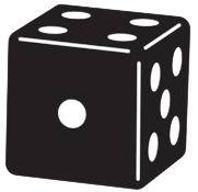
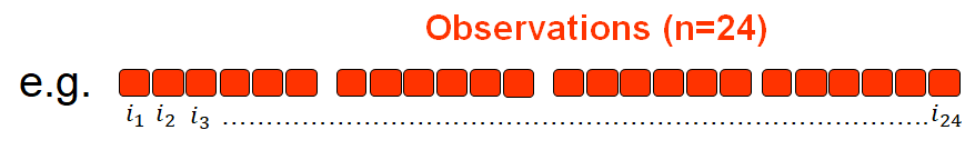
: \(\color{green}{Y}\) - We have data on a number \((n)\) of observations \(({i})\) (e.g. survey respondents; pupils; students; factory workers; events; etc.): \({i}_{1\dots{n}}\)
- We assume that observations are independent of each other (e.g. different respondents randomly sampled from a population)
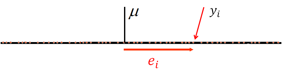
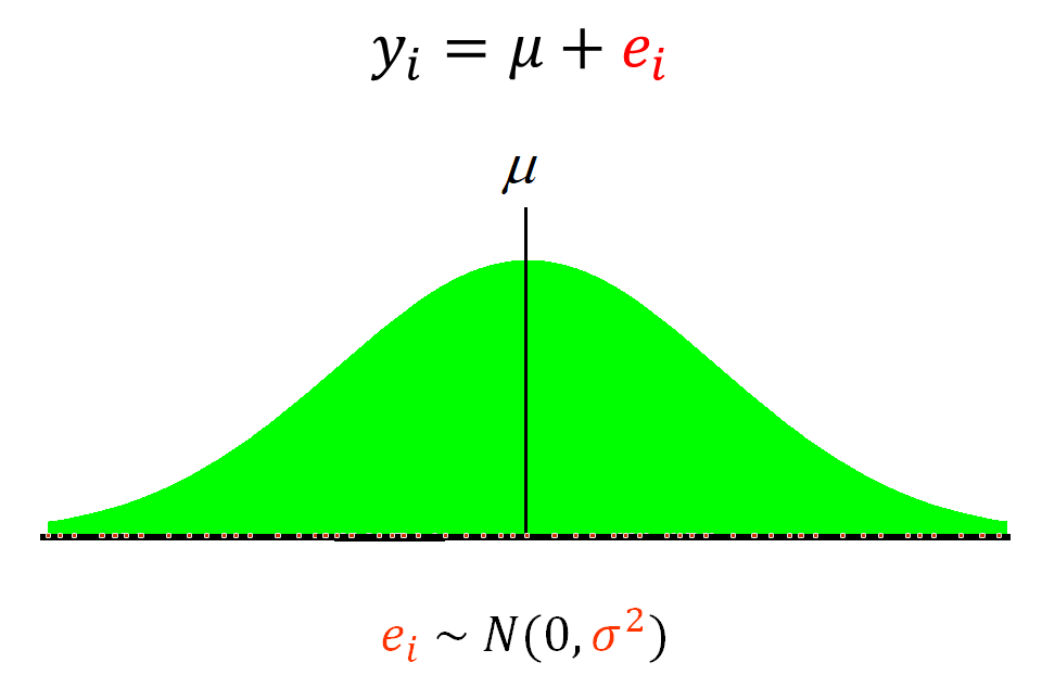
- The outcome measurement has a grand mean across all observations \((\mu)\), and each observation \((i)\) has some deviation (
error
) from this mean \((e_i)\) - \[ y_i = \mu + \color{red}{e_i} \]
A brief review of single-level regression
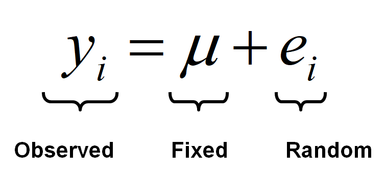
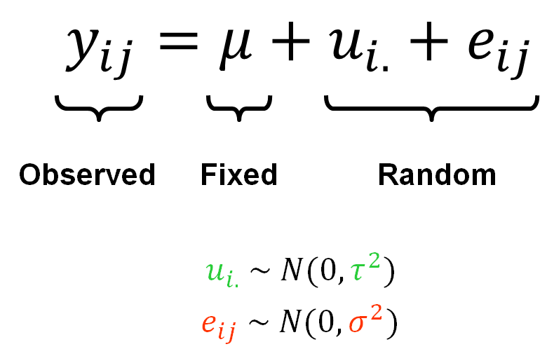
Observed part: our observation, outcome, estimate, etc.; the left-hand-side of the model
Fixed part: this can be a simple sample mean \((\mu)\) of a single measurement as in our basic example (e.g. a social trust scale), but it can also be a regression equation containing several predictor variables, as we have seen in previous weeks (e.g. \(b_0 + b_{1i}x_{1i} + b_{2i}x_{2i} \cdots b_{pi}x_{pi}\) for a model with \(p\) number of predictors/independent variables)
Random part: the deviations of the observations from the model mean
A brief review of single-level regression
- We also assume that the error term \((e)\) is Normally distributed around a mean of 0 and has some variance \((\sigma^2)\) that we are estimating
Multilevel models
Multilevel data
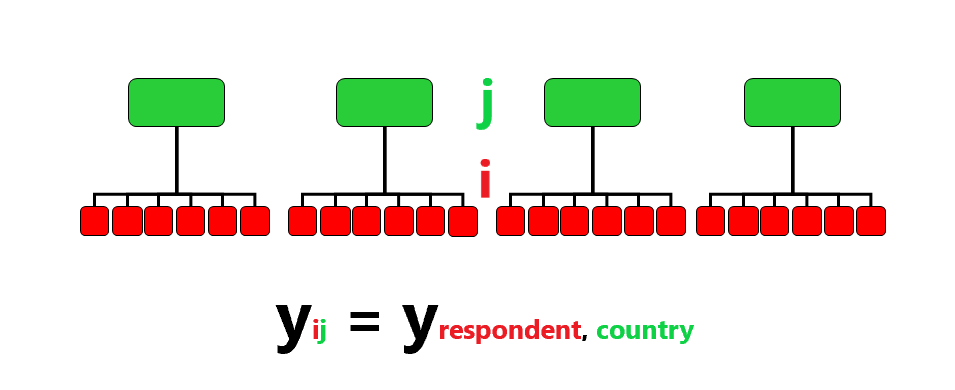
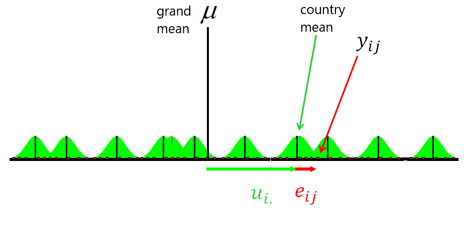
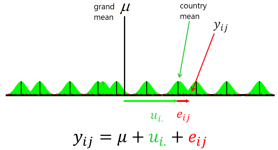
In our dataset we cannot assume that the observations are fully independent (or that the errors are independently distributed). We know that observations were sampled from within selected countries, so the countries are cluster variables that may have a group-level influence on the behaviour, opinions, conditions etc. of our individual observations.
Multilevel data
In our dataset we cannot assume that the observations are fully independent (or that the errors are independently distributed). We know that observations were sampled from within selected countries, so the countries are cluster variables that may have a group-level influence on the behaviour, opinions, conditions etc. of our individual observations.
Application: Österman (2021)