## Install first if not yet installed

library("tidyverse")
library("sjlabelled")
library("easystats")
library("ggformula")
library("ggeffects")
library("marginaleffects")
library("modelsummary")
library("gtsummary")
library("sjPlot")
library("lme4")              # for general hierarchical modelling
library("panelr")            # for time-series hierarchical data structures
library("plm")               # for time-series hierarchical data structures
library("pglm") # for time-series hierarchical data structuresWeek 6 Application Lab
Temporalities: Panel, longitudinal and time-series analysis
Aims
By the end of the session you will learn how to:
- fit random-intercepts and random coefficients models to hierarchical data that contains a temporal dimension
- use functions for modelling time-series data
Setup
In Week 1 you set up R and RStudio, and an RProject folder (we called it “HSS8005_labs”) with an .R script and a .qmd or .Rmd document in it (we called these “Lab_1”). Ideally, you saved this on a cloud drive so you can access it from any computer (e.g. OneDrive). You will be working in this folder.
Create a new Quarto markdown file (.qmd) for this session (e.g. “Lab_6.qmd”) and work in it to complete the exercises and report on your final analysis.
Packages
Exercise 1: longitudinal multi-level analysis
Data
Mitchell (2021) uses the European Social Survey (2002–2016) to test how differences in social trust, both within and between countries influence attitudes about immigrants. The ESS is a cross-national survey with representative samples of 34 countries, all of them are included in this study. Three items were included in each of the eight waves of the ESS to measure attitudes about immigrants:
- “Would you say it is generally bad or good for [country]’s economy that people come to live here from other countries?” (0= “Bad for the economy,” 10 = “Good for the economy”).
- “Would you say that [country]’s cultural life is generally undermined or enriched by people coming to live here from other countries?” (0 = “Cultural life undermined,” 10= “Cultural life enriched”).
- “Is [country] made a worse or a better place to live by people coming to live here from other countries?,” (0= “Worse place to live,” 10 = “Better place to live”).
An index was created by averaging responses to each of the three questions.
The main independent variable measures generalized trust. At the individual level, trust is measured through the question, “generally speaking, would you say that most people can be trusted, or that you can’t be too careful in dealing with people?” On a 10 point scale (0= “You cant be too careful,” 10= “most people can be trusted”). To isolate individuals’ trust levels in a way that is relative to the respondents’ country, responses were centred against the average level of generalized trust in that country at that time. This means that, the variable included in the analysis is the level of difference people say that they can trust others, compared to others in their country during the survey wave.
Due to the structure of the data, a multi-level modelling approach that nests respondents inside of country-years and counties was employed for this study. This allows for both the estimation of the relationship between contextual variables of interest and anti-immigrant attitudes both cross-sectionally and longitudinally. Since the responses to the surveys are in part dependent on the groups that the respondents belong, models that accommodate for this country and country-year grouping are better suited for this analysis than models with no grouping structure.
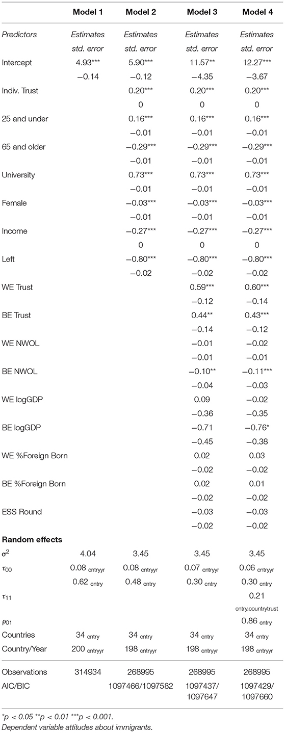
The analysis follows a model building approach where Model 1 is an “empty” model for the dependent variable and its nesting structure in the three level model. Model 2 tests the relationship between the individual level independent variables and the dependent variable measuring respondents’ attitudes about immigrants. Model 3 adds the country level independent variables, including country level social trust. In the first three models random intercepts are used in estimation, and Model 4 adds random slopes to the estimates in the three- level models. These models are presented in Table 1 of the article (see there).
Data import
We can load the dataset from the course website:
mitchell <- data_read("https://cgmoreh.github.io/HSS8005/data/mitchell2021.rds")Dataset structure
Columns/variables:
datawizard::data_peek(mitchell)| Data frame with 348104 rows and 70 variables | ||
|---|---|---|
| Variable | Type | Values |
| cntry | factor | Austria, Austria, Austria, Austria, ... |
| essround | numeric | 1, 1, 1, 1, 1, 1, 1, 1, 1, 1, 1, 1, ... |
| yrbrn | numeric | 1949, 1953, 1940, 1959, 1962, 1940, ... |
| brncntr | factor | 1, 1, 1, 1, 1, 1, 1, 1, 1, 1, 1, 1, ... |
| eisced | numeric | 0, 0, 0, 0, 0, 0, 0, 0, 0, 0, 0, 0, ... |
| gndr | factor | Female, Female, Male, Female, Male, ... |
| imsmetn | numeric | 1, 3, 2, 4, NA, 4, NA, 3, 2, NA, 2, ... |
| imdfetn | numeric | 2, 3, 2, 3, NA, 4, NA, 3, 2, NA, 2, ... |
| impcntr | numeric | 2, 3, 2, 4, NA, 4, NA, 3, 2, NA, 2, ... |
| imbgeco | numeric | 4, 10, 7, 10, NA, 5, 5, 8, 6, 5, 5, ... |
| imueclt | numeric | 9, 10, 5, 10, NA, 7, 5, 5, 5, 5, 3, ... |
| imwbcnt | numeric | 7, 5, 5, 10, NA, 5, 5, 5, 6, 5, 4, ... |
| ppltrst | numeric | 7, 6, 0, 8, 8, 0, 5, 7, 4, 6, 0, 0, ... |
| trstprl | numeric | 9, 0, 6, 8, 6, 0, 6, 5, 0, 2, 5, 0, ... |
| trstlgl | factor | 10, 8, 4, 10, 7, 5, 6, 7, 3, 2, 5, ... |
| trstplc | factor | 10, 5, 8, 9, 4, 6, 6, 8, 5, 7, 3, ... |
| trstplt | numeric | 0, 0, 2, 4, 4, 0, 5, 3, 5, 0, 3, 0, ... |
| trstprt | factor | NA, NA, NA, NA, NA, NA, NA, NA, NA, ... |
| trstep | factor | NA, 0, 7, 7, 4, 2, 5, 2, NA, 0, 3, ... |
| trstun | factor | 9, 6, NA, 8, 5, NA, NA, 0, NA, 0, ... |
| hincfel | factor | 1, 3, 2, 1, 1, 3, 2, 1, 2, NA, 2, ... |
| lrscale | numeric | 6, 6, 5, 5, 5, NA, NA, 5, 5, 5, 5, ... |
| dweight | numeric | 0.945200026035309, ... |
| edulvlb | numeric | NA, NA, NA, NA, NA, NA, NA, NA, NA, ... |
| year | numeric | 2002, 2002, 2002, 2002, 2002, 2002, ... |
| immsent | numeric | 1.66666666666667, 3, 2, ... |
| na.rm | logical | TRUE, TRUE, TRUE, TRUE, TRUE, TRUE, ... |
| immatt | numeric | 6.66666666666667, 8.33333333333333, ... |
| insttrust | numeric | 4.5, 0, 4, 6, 5, 0, 5.5, 4, 2.5, 1, ... |
| age | numeric | 53, 49, 62, 43, 40, 62, 74, 46, 51, ... |
| university | numeric | 0, 0, 0, 0, 0, 0, 0, 0, 0, 0, 0, 0, ... |
| young | numeric | 0, 0, 0, 0, 0, 0, 0, 0, 0, 0, 0, 0, ... |
| old | numeric | 0, 0, 0, 0, 0, 0, 1, 0, 0, 0, 0, 0, ... |
| cntryyr | factor | 10001, 10001, 10001, 10001, 10001, ... |
| countrytrust | numeric | 5.06821221578243, 5.06821221578243, ... |
| countryatt | numeric | 5.39790486003778, 5.39790486003778, ... |
| countryinst | numeric | 4.29170506912442, 4.29170506912442, ... |
| iso2c | character | AT, AT, AT, AT, AT, AT, AT, AT, AT, ... |
| iso3c | character | AUT, AUT, AUT, AUT, AUT, AUT, AUT, ... |
| NY.GDP.PCAP.PP.KD | numeric | 47419.2784117541, 47419.2784117541, ... |
| SL.UEM.TOTL.NE.ZS | numeric | 4.86, 4.86, 4.86, 4.86, 4.86, 4.86, ... |
| SM.POP.TOTL.ZS | numeric | NA, NA, NA, NA, NA, NA, NA, NA, NA, ... |
| SL.TLF.TOTL.FE.ZS | numeric | 44.6880614869325, 44.6880614869325, ... |
| SP.POP.65UP.TO.ZS | numeric | 15.433002037878, 15.433002037878, ... |
| CC.EST | numeric | 1.91515922546387, 1.91515922546387, ... |
| PctFB | numeric | 12.9461819335583, 12.9461819335583, ... |
| PctFB2000 | numeric | 12.3781065532679, 12.3781065532679, ... |
| PctFB2016 | numeric | 17.465726250517, 17.465726250517, ... |
| FBchange | numeric | 5.0876196972491, 5.0876196972491, ... |
| GDP | numeric | 47419.2784117541, 47419.2784117541, ... |
| UNEMP | numeric | 4.86, 4.86, 4.86, 4.86, 4.86, 4.86, ... |
| AGED | numeric | 15.433002037878, 15.433002037878, ... |
| CORRUPT | numeric | 1.91515922546387, 1.91515922546387, ... |
| FEMLAB | numeric | 44.6880614869325, 44.6880614869325, ... |
| countrytrustM | numeric | 5.14513967632203, 5.14513967632203, ... |
| countryattM | numeric | 4.73865058595972, 4.73865058595972, ... |
| PctFBM | numeric | 14.8237866389353, 14.8237866389353, ... |
| GDPM | numeric | 50454.1491777596, 50454.1491777596, ... |
| countryinstM | numeric | 4.17517334744597, 4.17517334744597, ... |
| ppltrustc | numeric | 5.07153356197942, 5.07153356197942, ... |
| ppltrustd | numeric | 1.92846643802058, ... |
| countrytrustD | numeric | -0.0769274605395944, ... |
| countryinstD | numeric | 0.116531721678455, ... |
| PctFBD | numeric | -1.87760470537692, ... |
| lGDP | numeric | 10.7667841425436, 10.7667841425436, ... |
| lGDPM | numeric | 10.8288202657649, 10.8288202657649, ... |
| lGDPD | numeric | -0.0620361232213025, ... |
| mean_NWOL | numeric | 12.3535519125683, 12.3535519125683, ... |
| nwolM | numeric | 3.88027195977658, 3.88027195977658, ... |
| nwolD | numeric | -2.64491676851975, ... |
Rows/cases:
gt::gt_preview(mitchell, top_n = 5, bottom_n = 5)| cntry | essround | yrbrn | brncntr | eisced | gndr | imsmetn | imdfetn | impcntr | imbgeco | imueclt | imwbcnt | ppltrst | trstprl | trstlgl | trstplc | trstplt | trstprt | trstep | trstun | hincfel | lrscale | dweight | edulvlb | year | immsent | na.rm | immatt | insttrust | age | university | young | old | cntryyr | countrytrust | countryatt | countryinst | iso2c | iso3c | NY.GDP.PCAP.PP.KD | SL.UEM.TOTL.NE.ZS | SM.POP.TOTL.ZS | SL.TLF.TOTL.FE.ZS | SP.POP.65UP.TO.ZS | CC.EST | PctFB | PctFB2000 | PctFB2016 | FBchange | GDP | UNEMP | AGED | CORRUPT | FEMLAB | countrytrustM | countryattM | PctFBM | GDPM | countryinstM | ppltrustc | ppltrustd | countrytrustD | countryinstD | PctFBD | lGDP | lGDPM | lGDPD | mean_NWOL | nwolM | nwolD | |
|---|---|---|---|---|---|---|---|---|---|---|---|---|---|---|---|---|---|---|---|---|---|---|---|---|---|---|---|---|---|---|---|---|---|---|---|---|---|---|---|---|---|---|---|---|---|---|---|---|---|---|---|---|---|---|---|---|---|---|---|---|---|---|---|---|---|---|---|---|---|---|
| 1 | Austria | 1 | 1949 | 1 | 0 | Female | 1 | 2 | 2 | 4 | 9 | 7 | 7 | 9 | 10 | 10 | 0 | NA | NA | 9 | 1 | 6 | 0.9452 | NA | 2002 | 1.666667 | TRUE | 6.666667 | 4.5 | 53 | 0 | 0 | 0 | 10001 | 5.068212 | 5.397905 | 4.291705 | AT | AUT | 47419.28 | 4.86 | NA | 44.68806 | 15.43300 | 1.9151592 | 12.9461819 | 12.3781066 | 17.465726 | 5.0876197 | 47419.28 | 4.86 | 15.43300 | 1.9151592 | 44.68806 | 5.145140 | 4.738651 | 14.8237866 | 50454.15 | 4.175173 | 5.071534 | 1.92846644 | -0.07692746 | 0.1165317 | -1.87760471 | 10.766784 | 10.828820 | -0.06203612 | 12.35355 | 3.880272 | -2.64491677 |
| 2 | Austria | 1 | 1953 | 1 | 0 | Female | 3 | 3 | 3 | 10 | 10 | 5 | 6 | 0 | 8 | 5 | 0 | NA | 0 | 6 | 3 | 6 | 0.4726 | NA | 2002 | 3.000000 | TRUE | 8.333333 | 0.0 | 49 | 0 | 0 | 0 | 10001 | 5.068212 | 5.397905 | 4.291705 | AT | AUT | 47419.28 | 4.86 | NA | 44.68806 | 15.43300 | 1.9151592 | 12.9461819 | 12.3781066 | 17.465726 | 5.0876197 | 47419.28 | 4.86 | 15.43300 | 1.9151592 | 44.68806 | 5.145140 | 4.738651 | 14.8237866 | 50454.15 | 4.175173 | 5.071534 | 0.92846644 | -0.07692746 | 0.1165317 | -1.87760471 | 10.766784 | 10.828820 | -0.06203612 | 12.35355 | 3.880272 | -2.64491677 |
| 3 | Austria | 1 | 1940 | 1 | 0 | Male | 2 | 2 | 2 | 7 | 5 | 5 | 0 | 6 | 4 | 8 | 2 | NA | 7 | NA | 2 | 5 | 0.9452 | NA | 2002 | 2.000000 | TRUE | 5.666667 | 4.0 | 62 | 0 | 0 | 0 | 10001 | 5.068212 | 5.397905 | 4.291705 | AT | AUT | 47419.28 | 4.86 | NA | 44.68806 | 15.43300 | 1.9151592 | 12.9461819 | 12.3781066 | 17.465726 | 5.0876197 | 47419.28 | 4.86 | 15.43300 | 1.9151592 | 44.68806 | 5.145140 | 4.738651 | 14.8237866 | 50454.15 | 4.175173 | 5.071534 | -5.07153356 | -0.07692746 | 0.1165317 | -1.87760471 | 10.766784 | 10.828820 | -0.06203612 | 12.35355 | 3.880272 | -2.64491677 |
| 4 | Austria | 1 | 1959 | 1 | 0 | Female | 4 | 3 | 4 | 10 | 10 | 10 | 8 | 8 | 10 | 9 | 4 | NA | 7 | 8 | 1 | 5 | 0.9452 | NA | 2002 | 3.666667 | TRUE | 10.000000 | 6.0 | 43 | 0 | 0 | 0 | 10001 | 5.068212 | 5.397905 | 4.291705 | AT | AUT | 47419.28 | 4.86 | NA | 44.68806 | 15.43300 | 1.9151592 | 12.9461819 | 12.3781066 | 17.465726 | 5.0876197 | 47419.28 | 4.86 | 15.43300 | 1.9151592 | 44.68806 | 5.145140 | 4.738651 | 14.8237866 | 50454.15 | 4.175173 | 5.071534 | 2.92846644 | -0.07692746 | 0.1165317 | -1.87760471 | 10.766784 | 10.828820 | -0.06203612 | 12.35355 | 3.880272 | -2.64491677 |
| 5 | Austria | 1 | 1962 | 1 | 0 | Male | NA | NA | NA | NA | NA | NA | 8 | 6 | 7 | 4 | 4 | NA | 4 | 5 | 1 | 5 | 1.8905 | NA | 2002 | NA | TRUE | NA | 5.0 | 40 | 0 | 0 | 0 | 10001 | 5.068212 | 5.397905 | 4.291705 | AT | AUT | 47419.28 | 4.86 | NA | 44.68806 | 15.43300 | 1.9151592 | 12.9461819 | 12.3781066 | 17.465726 | 5.0876197 | 47419.28 | 4.86 | 15.43300 | 1.9151592 | 44.68806 | 5.145140 | 4.738651 | 14.8237866 | 50454.15 | 4.175173 | 5.071534 | 2.92846644 | -0.07692746 | 0.1165317 | -1.87760471 | 10.766784 | 10.828820 | -0.06203612 | 12.35355 | 3.880272 | -2.64491677 |
| 6..348099 | ||||||||||||||||||||||||||||||||||||||||||||||||||||||||||||||||||||||
| 348100 | Romania | 3 | 1949 | 1 | 4 | Female | 3 | 2 | 2 | 6 | 6 | 5 | 3 | 4 | 6 | 5 | 3 | 3 | 7 | 6 | 2 | 8 | NA | NA | 2006 | 2.333333 | TRUE | 5.666667 | 3.5 | 57 | 0 | 0 | 0 | 250003 | 4.073251 | 5.912133 | 3.064788 | RO | ROU | 18325.74 | 7.27 | NA | 45.30711 | 14.93628 | -0.2091585 | 0.6961542 | 0.5736994 | 1.163135 | 0.5894354 | 18325.74 | 7.27 | 14.93628 | -0.2091585 | 45.30711 | 3.936573 | 5.627671 | 0.7140428 | 20226.96 | 3.242876 | 4.075937 | -1.07593735 | 0.13667890 | -0.1780883 | -0.01788859 | 9.816062 | 9.914771 | -0.09870970 | 38.55587 | 3.840235 | 0.01535259 |
| 348101 | Romania | 3 | 1958 | 1 | 5 | Male | 3 | 2 | 1 | 7 | 6 | 7 | 4 | 3 | 8 | 7 | 4 | 2 | 6 | 6 | 2 | 8 | NA | NA | 2006 | 2.000000 | TRUE | 6.666667 | 3.5 | 48 | 0 | 0 | 0 | 250003 | 4.073251 | 5.912133 | 3.064788 | RO | ROU | 18325.74 | 7.27 | NA | 45.30711 | 14.93628 | -0.2091585 | 0.6961542 | 0.5736994 | 1.163135 | 0.5894354 | 18325.74 | 7.27 | 14.93628 | -0.2091585 | 45.30711 | 3.936573 | 5.627671 | 0.7140428 | 20226.96 | 3.242876 | 4.075937 | -0.07593735 | 0.13667890 | -0.1780883 | -0.01788859 | 9.816062 | 9.914771 | -0.09870970 | 38.55587 | 3.840235 | 0.01535259 |
| 348102 | Romania | 3 | 1944 | 1 | 3 | Male | 2 | 2 | 2 | 6 | 7 | 7 | 5 | 3 | 4 | 5 | 2 | 3 | 6 | 6 | 2 | 2 | NA | NA | 2006 | 2.000000 | TRUE | 6.666667 | 2.5 | 62 | 0 | 0 | 0 | 250003 | 4.073251 | 5.912133 | 3.064788 | RO | ROU | 18325.74 | 7.27 | NA | 45.30711 | 14.93628 | -0.2091585 | 0.6961542 | 0.5736994 | 1.163135 | 0.5894354 | 18325.74 | 7.27 | 14.93628 | -0.2091585 | 45.30711 | 3.936573 | 5.627671 | 0.7140428 | 20226.96 | 3.242876 | 4.075937 | 0.92406265 | 0.13667890 | -0.1780883 | -0.01788859 | 9.816062 | 9.914771 | -0.09870970 | 38.55587 | 3.840235 | 0.01535259 |
| 348103 | Romania | 3 | 1948 | 1 | 3 | Male | 3 | 3 | 2 | 7 | 5 | 4 | 4 | 3 | 7 | 8 | 4 | 2 | 6 | 8 | 3 | 7 | NA | NA | 2006 | 2.666667 | TRUE | 5.333333 | 3.5 | 58 | 0 | 0 | 0 | 250003 | 4.073251 | 5.912133 | 3.064788 | RO | ROU | 18325.74 | 7.27 | NA | 45.30711 | 14.93628 | -0.2091585 | 0.6961542 | 0.5736994 | 1.163135 | 0.5894354 | 18325.74 | 7.27 | 14.93628 | -0.2091585 | 45.30711 | 3.936573 | 5.627671 | 0.7140428 | 20226.96 | 3.242876 | 4.075937 | -0.07593735 | 0.13667890 | -0.1780883 | -0.01788859 | 9.816062 | 9.914771 | -0.09870970 | 38.55587 | 3.840235 | 0.01535259 |
| 348104 | Romania | 3 | 1923 | 1 | 6 | Female | 3 | 3 | 2 | 8 | 7 | 7 | 4 | 5 | 7 | 8 | 4 | 3 | 6 | 5 | 2 | 4 | NA | NA | 2006 | 2.666667 | TRUE | 7.333333 | 4.5 | 83 | 1 | 0 | 1 | 250003 | 4.073251 | 5.912133 | 3.064788 | RO | ROU | 18325.74 | 7.27 | NA | 45.30711 | 14.93628 | -0.2091585 | 0.6961542 | 0.5736994 | 1.163135 | 0.5894354 | 18325.74 | 7.27 | 14.93628 | -0.2091585 | 45.30711 | 3.936573 | 5.627671 | 0.7140428 | 20226.96 | 3.242876 | 4.075937 | -0.07593735 | 0.13667890 | -0.1780883 | -0.01788859 | 9.816062 | 9.914771 | -0.09870970 | 38.55587 | 3.840235 | 0.01535259 |
Variable distribution:
datawizard::describe_distribution(mitchell)| Variable | Mean | SD | IQR | Min | Max | Skewness | Kurtosis | n | n_Missing |
|---|---|---|---|---|---|---|---|---|---|
| essround | 4.46 | 2.20 | 3.00 | 1.00 | 8.00 | 0.04 | -1.12 | 348104 | 0 |
| yrbrn | 1961.48 | 18.98 | 30.00 | 1885.00 | 2002.00 | -0.10 | -0.83 | 346771 | 1333 |
| eisced | 3.10 | 3.04 | 4.00 | 0.00 | 55.00 | 8.14 | 136.22 | 347195 | 909 |
| imsmetn | 2.79 | 0.89 | 1.00 | 1.00 | 4.00 | -0.35 | -0.61 | 335619 | 12485 |
| imdfetn | 2.47 | 0.91 | 1.00 | 1.00 | 4.00 | -0.04 | -0.80 | 334870 | 13234 |
| impcntr | 2.39 | 0.92 | 1.00 | 1.00 | 4.00 | 0.05 | -0.87 | 333250 | 14854 |
| imbgeco | 4.76 | 2.45 | 4.00 | 0.00 | 10.00 | -0.13 | -0.50 | 330181 | 17923 |
| imueclt | 5.37 | 2.57 | 3.00 | 0.00 | 10.00 | -0.26 | -0.55 | 330897 | 17207 |
| imwbcnt | 4.72 | 2.31 | 3.00 | 0.00 | 10.00 | -0.09 | -0.21 | 329827 | 18277 |
| ppltrst | 4.96 | 2.48 | 4.00 | 0.00 | 10.00 | -0.26 | -0.65 | 346824 | 1280 |
| trstprl | 4.30 | 2.60 | 4.00 | 0.00 | 10.00 | -0.03 | -0.80 | 339363 | 8741 |
| trstplt | 3.44 | 2.39 | 4.00 | 0.00 | 10.00 | 0.18 | -0.82 | 341446 | 6658 |
| lrscale | 5.16 | 2.23 | 3.00 | 0.00 | 10.00 | -0.04 | 0.03 | 298485 | 49619 |
| dweight | 1.00 | 0.43 | 0.22 | 1.60e-03 | 6.21 | 2.12 | 11.20 | 344221 | 3883 |
| edulvlb | Inf | -Inf | 0 | 348104 | |||||
| year | 2008.92 | 4.40 | 6.00 | 2002.00 | 2016.00 | 0.04 | -1.12 | 348104 | 0 |
| immsent | 2.55 | 0.81 | 1.00 | 1.00 | 4.00 | -0.08 | -0.55 | 328190 | 19914 |
| immatt | 4.96 | 2.15 | 2.67 | 0.00 | 10.00 | -0.25 | -0.20 | 314934 | 33170 |
| insttrust | 3.87 | 2.32 | 3.50 | 0.00 | 10.00 | 0.01 | -0.80 | 336632 | 11472 |
| age | 47.83 | 18.45 | 29.00 | 16.00 | 100.00 | 0.12 | -0.93 | 342631 | 5473 |
| university | 0.16 | 0.37 | 0.00 | 0.00 | 1.00 | 1.82 | 1.31 | 347195 | 909 |
| young | 0.14 | 0.35 | 0.00 | 0.00 | 1.00 | 2.05 | 2.22 | 342631 | 5473 |
| old | 0.22 | 0.41 | 0.00 | 0.00 | 1.00 | 1.39 | -0.08 | 342631 | 5473 |
| countrytrust | 4.95 | 0.94 | 1.31 | 2.29 | 7.02 | 0.28 | -0.37 | 348104 | 0 |
| countryatt | 5.03 | 0.75 | 0.99 | 3.02 | 7.01 | -0.33 | -0.31 | 348104 | 0 |
| countryinst | 3.88 | 1.05 | 1.54 | 1.51 | 6.09 | 3.93e-03 | -0.60 | 348104 | 0 |
| NY.GDP.PCAP.PP.KD | 39828.31 | 14288.90 | 20251.52 | 10902.04 | 1.08e+05 | 0.58 | 1.76 | 329121 | 18983 |
| SL.UEM.TOTL.NE.ZS | 8.19 | 3.87 | 4.45 | 2.55 | 24.79 | 1.62 | 3.55 | 329121 | 18983 |
| SM.POP.TOTL.ZS | 10.70 | 5.97 | 7.22 | 1.03 | 26.50 | 0.61 | 0.76 | 45140 | 302964 |
| SL.TLF.TOTL.FE.ZS | 46.15 | 2.25 | 2.24 | 38.93 | 51.61 | -0.59 | 1.11 | 329121 | 18983 |
| SP.POP.65UP.TO.ZS | 16.32 | 2.60 | 3.17 | 9.96 | 22.28 | -0.47 | -0.19 | 329121 | 18983 |
| CC.EST | 1.16 | 0.91 | 1.38 | -1.13 | 2.46 | -0.73 | -0.21 | 329121 | 18983 |
| PctFB | 10.83 | 6.18 | 6.31 | 0.70 | 32.73 | 0.90 | 1.44 | 329121 | 18983 |
| PctFB2000 | 9.07 | 6.34 | 6.91 | 0.54 | 32.04 | 1.64 | 3.43 | 329121 | 18983 |
| PctFB2016 | 11.96 | 6.60 | 6.79 | 1.16 | 43.96 | 1.14 | 3.54 | 329121 | 18983 |
| FBchange | 2.89 | 3.41 | 4.06 | -5.84 | 11.92 | -0.23 | 0.06 | 329121 | 18983 |
| GDP | 39828.31 | 14288.90 | 20251.52 | 10902.04 | 1.08e+05 | 0.58 | 1.76 | 329121 | 18983 |
| UNEMP | 8.19 | 3.87 | 4.45 | 2.55 | 24.79 | 1.62 | 3.55 | 329121 | 18983 |
| AGED | 16.32 | 2.60 | 3.17 | 9.96 | 22.28 | -0.47 | -0.19 | 329121 | 18983 |
| CORRUPT | 1.16 | 0.91 | 1.38 | -1.13 | 2.46 | -0.73 | -0.21 | 329121 | 18983 |
| FEMLAB | 46.15 | 2.25 | 2.24 | 38.93 | 51.61 | -0.59 | 1.11 | 329121 | 18983 |
| countrytrustM | 4.96 | 0.94 | 1.29 | 2.60 | 6.96 | 0.34 | -0.40 | 348104 | 0 |
| countryattM | 4.95 | 0.72 | 0.90 | 3.22 | 6.65 | -0.30 | -0.25 | 348104 | 0 |
| PctFBM | 10.83 | 6.05 | 6.32 | 0.71 | 32.56 | 0.90 | 1.53 | 329121 | 18983 |
| GDPM | 39828.31 | 14056.42 | 18928.19 | 12418.04 | 1.06e+05 | 0.57 | 1.80 | 329121 | 18983 |
| countryinstM | 3.88 | 0.96 | 1.27 | 1.95 | 5.77 | 0.25 | -0.67 | 348104 | 0 |
| ppltrustc | 4.96 | 0.96 | 1.31 | 2.29 | 7.08 | 0.28 | -0.40 | 348104 | 0 |
| ppltrustd | -8.56e-18 | 2.29 | 3.15 | -7.08 | 7.71 | -0.16 | -0.28 | 346824 | 1280 |
| countrytrustD | -9.79e-03 | 0.18 | 0.24 | -0.41 | 0.54 | 0.48 | 0.28 | 348104 | 0 |
| countryinstD | -4.23e-17 | 0.42 | 0.52 | -1.52 | 1.62 | -0.02 | 1.63 | 348104 | 0 |
| PctFBD | -8.04e-16 | 1.28 | 1.25 | -4.99 | 4.10 | -0.22 | 1.57 | 329121 | 18983 |
| lGDP | 10.52 | 0.39 | 0.54 | 9.30 | 11.59 | -0.66 | 0.34 | 329121 | 18983 |
| lGDPM | 10.52 | 0.38 | 0.51 | 9.43 | 11.57 | -0.64 | 0.30 | 329121 | 18983 |
| lGDPD | -2.56e-03 | 0.07 | 0.08 | -0.30 | 0.24 | -0.54 | 2.60 | 329121 | 18983 |
| mean_NWOL | 35.66 | 39.98 | 39.36 | 0.00 | 210.16 | 2.06 | 4.72 | 348104 | 0 |
| nwolM | 3.57 | 3.43 | 2.58 | 0.16 | 15.15 | 1.78 | 2.75 | 348104 | 0 |
| nwolD | 4.50e-17 | 2.05 | 1.65 | -11.12 | 6.11 | -0.68 | 6.70 | 348104 | 0 |
Grouping variables:
We can check the number of unique (or distinct) values in our “grouping” variables with either the insight::n_unique() function (loaded with easystats) or dplyr::n_distinct() (loaded with tidyverse). Below we use the former and concatenate the numeric output with a textual description of its meaning (using the paste() function):
paste("Number of countries:", n_unique(mitchell$cntry))
paste("Number of ESS survey rounds:", n_unique(mitchell$essround))
paste("Number of country/survey-round pairs:", n_unique(mitchell$cntryyr))
[1] "Number of countries: 34"
[1] "Number of ESS survey rounds: 8"
[1] "Number of country/survey-round pairs: 200"We can see that 200 is smaller than 34 \(\times\) 8 \(=\) 272, which means that not every country in the dataset participated in all of the survey rounds. We can cross-tabulate the cntry and the essround variables to get a matrix of the sample size in each country and round, with 0 representing the missing country-rounds:
data_tabulate(mitchell,
              "cntry",
              by = "essround")

# or #

data_tabulate(mitchell$cntry,
mitchell$essround)| `cntry` by `essround` | 1 | 2 | 3 | 4 | 5 | 6 | 7 | 8 | Total |
|---|---|---|---|---|---|---|---|---|---|
| Austria | 2053 | 2074 | 2236 | 0 | 0 | 0 | 1584 | 1804 | 9,751 |
| Belgium | 1739 | 1619 | 1645 | 1586 | 1516 | 1606 | 1542 | 1507 | 12,760 |
| Bulgaria | 0 | 0 | 1387 | 2210 | 2412 | 2247 | 0 | 0 | 8,256 |
| Croatia | 0 | 0 | 0 | 1353 | 1474 | 0 | 0 | 0 | 2,827 |
| Cyprus | 0 | 0 | 945 | 1119 | 1016 | 991 | 0 | 0 | 4,071 |
| Czech Republic | 1297 | 2890 | 0 | 1976 | 2339 | 1944 | 2102 | 2216 | 14,764 |
| Denmark | 1422 | 1415 | 1403 | 1510 | 1475 | 1536 | 1382 | 0 | 10,143 |
| Estonia | 0 | 1615 | 1199 | 1305 | 1517 | 1991 | 1649 | 1723 | 10,999 |
| Finland | 1937 | 1983 | 1838 | 2139 | 1813 | 2103 | 1987 | 1848 | 15,648 |
| France | 1353 | 1670 | 1791 | 1911 | 1573 | 1760 | 1694 | 1857 | 13,609 |
| Germany | 2705 | 2625 | 2687 | 2518 | 2743 | 2658 | 2745 | 2555 | 21,236 |
| Greece | 2302 | 2164 | 0 | 1950 | 2447 | 0 | 0 | 0 | 8,863 |
| Hungary | 1645 | 1465 | 1484 | 1514 | 1518 | 1989 | 1671 | 1587 | 12,873 |
| Iceland | 0 | 554 | 0 | 0 | 0 | 707 | 0 | 825 | 2,086 |
| Ireland | 1890 | 2138 | 1561 | 1479 | 2170 | 2244 | 2075 | 2304 | 15,861 |
| Israel | 1626 | 0 | 0 | 1588 | 1529 | 1725 | 1738 | 1817 | 10,023 |
| Italy | 1181 | 1494 | 0 | 0 | 0 | 887 | 0 | 2392 | 5,954 |
| Latvia | 0 | 0 | 1753 | 1706 | 0 | 0 | 0 | 0 | 3,459 |
| Lithuania | 0 | 0 | 0 | 0 | 1592 | 2047 | 2175 | 2067 | 7,881 |
| Luxembourg | 1069 | 1147 | 0 | 0 | 0 | 0 | 0 | 0 | 2,216 |
| Netherlands | 2207 | 1717 | 1711 | 1610 | 1688 | 1677 | 1736 | 1546 | 13,892 |
| Norway | 1903 | 1632 | 1625 | 1418 | 1373 | 1421 | 1267 | 1375 | 12,014 |
| Poland | 2079 | 1697 | 1696 | 1596 | 1723 | 1872 | 1598 | 1680 | 13,941 |
| Portugal | 1421 | 1932 | 2078 | 2229 | 2004 | 2019 | 1170 | 1172 | 14,025 |
| Romania | 0 | 0 | 2130 | 2088 | 0 | 0 | 0 | 0 | 4,218 |
| Russian Federation | 0 | 0 | 2280 | 2376 | 2435 | 2334 | 0 | 2303 | 11,728 |
| Slovak Republic | 0 | 1465 | 1703 | 1760 | 1802 | 1815 | 0 | 0 | 8,545 |
| Slovenia | 1374 | 1320 | 1362 | 1178 | 1280 | 1144 | 1124 | 1183 | 9,965 |
| Spain | 1648 | 1545 | 1730 | 2341 | 1693 | 1671 | 1756 | 1749 | 14,133 |
| Sweden | 1785 | 1762 | 1710 | 1616 | 1324 | 1613 | 1554 | 1366 | 12,730 |
| Switzerland | 1696 | 1748 | 1464 | 1392 | 1155 | 1157 | 1139 | 1103 | 10,854 |
| Turkey | 0 | 1830 | 0 | 2389 | 0 | 0 | 0 | 0 | 4,219 |
| Ukraine | 0 | 1763 | 1759 | 1654 | 1717 | 2006 | 0 | 0 | 8,899 |
| United Kingdom | 1860 | 1724 | 2158 | 2106 | 2151 | 2020 | 1950 | 1692 | 15,661 |
| Total | 38,192 | 44,988 | 43,335 | 51,617 | 47,479 | 47,184 | 35,638 | 39,671 | 348,104 |
Temporal structure
We can explore visually the distribution of the core variable of interest (ppltrst) across the grouping factors.
ggplot(mitchell, aes(x = year, countrytrustD)) +
  theme_bw() +
  theme(axis.title.y = element_blank(),
        panel.grid.major = element_blank(),
        panel.grid.minor = element_blank()
        ) +
  facet_wrap(vars(cntry)) +
  geom_smooth(method = lm, se = FALSE, alpha = 0.5) +
  geom_line() +
  geom_point(shape = 1, alpha = 0.5)
Model 1: null models without predictors
m1  <- lmer(immatt~ 1 +
            (1|cntry/cntryyr), data=mitchell)

m1.1 <- lmer(immatt~ 1 +
              (1|cntry), data=mitchell)

m1.2 <- lmer(immatt~ 1 +
              (1|cntryyr), data=mitchell)

m1.3 <- lmer(immatt~ 1 +
              (1|cntry) +
              (1|cntry:cntryyr),
            data=mitchell)

m1.4 <- lmer(immatt~ 1 +
              (1|cntry) +
              (1|cntryyr:cntry),
            data=mitchell)

modelsummary::modelsummary(list("cntry/cntryyr" = m1, m1.1, m1.2, m1.3, "cntry+cntryyr:cntry" = m1.4))| cntry/cntryyr | cntry+cntryyr:cntry | ||||
|---|---|---|---|---|---|
| (Intercept) | 4.926 | 4.918 | 4.990 | 4.926 | 4.926 |
| (0.137) | (0.138) | (0.054) | (0.137) | (0.137) | |
| SD (Observations) | 2.009 | 2.025 | 2.009 | 2.009 | 2.009 |
| SD (Intercept cntry) | 0.786 | 0.804 | 0.786 | 0.786 | |
| SD (Intercept cntryyrcntry) | 0.280 | 0.280 | |||
| SD (Intercept cntryyr) | 0.763 | ||||
| SD (Intercept cntrycntryyr) | 0.280 | ||||
| Num.Obs. | 314934 | 314934 | 314934 | 314934 | 314934 |
| R2 Marg. | 0.000 | 0.000 | 0.000 | 0.000 | 0.000 |
| R2 Cond. | 0.147 | 0.136 | 0.126 | 0.147 | 0.147 |
| AIC | 1334097.2 | 1338521.2 | 1334365.6 | 1334097.2 | 1334097.2 |
| BIC | 1334139.9 | 1338553.2 | 1334397.6 | 1334139.9 | 1334139.9 |
| ICC | 0.1 | 0.1 | 0.1 | 0.1 | 0.1 |
| RMSE | 2.01 | 2.03 | 2.01 | 2.01 | 2.01 |
Model 2: individual level variables
m2 <- lmer(immatt ~ ppltrustd + young + old + university + gndr + hincfel + lrscale +
             (1|cntry) +
             (1|cntryyr),
           data=mitchell)
Model 3: contextual-level variables
m3 <- lmer(immatt ~ ppltrustd + young + old + university + gndr + hincfel + lrscale +
           countrytrustD + countrytrustM + nwolD + nwolM + lGDPD +
           lGDPM + PctFBD + PctFBM + essround +
           (1|cntry) +
           (1|cntryyr),
         data=mitchell)
Model 4: random slopes for between country trust
# due to convergence issues the REML=FALSE but the estimates are the same
m4 <- lmer(immatt~  ppltrustd + young + old + university + gndr + hincfel + lrscale +
           countrytrustD + countrytrustM + nwolD + nwolM + lGDPD +
           lGDPM + PctFBD + PctFBM + essround +
           (countrytrustD|cntry) +
           (1|cntryyr),
         data=mitchell)
Model comparison
We can use the same modelsummary() function we have already used before:
modelsummary::modelsummary(list(m1, m2, m3, m4))| (1) | (2) | (3) | (4) | |
|---|---|---|---|---|
| (Intercept) | 4.926 | 5.603 | 10.450 | 11.752 |
| (0.137) | (0.122) | (4.458) | (4.123) | |
| ppltrustd | 0.199 | 0.201 | 0.201 | |
| (0.002) | (0.002) | (0.002) | ||
| young | 0.157 | 0.140 | 0.140 | |
| (0.011) | (0.011) | (0.011) | ||
| old | -0.288 | -0.284 | -0.284 | |
| (0.009) | (0.009) | (0.009) | ||
| university | 0.728 | 0.734 | 0.734 | |
| (0.010) | (0.010) | (0.010) | ||
| gndrMale | -0.028 | -0.039 | -0.039 | |
| (0.007) | (0.007) | (0.007) | ||
| hincfel2 | -0.287 | -0.288 | -0.288 | |
| (0.009) | (0.009) | (0.009) | ||
| hincfel3 | -0.544 | -0.544 | -0.544 | |
| (0.012) | (0.012) | (0.012) | ||
| hincfel4 | -0.817 | -0.820 | -0.820 | |
| (0.017) | (0.018) | (0.018) | ||
| lrscale | -0.080 | -0.087 | -0.087 | |
| (0.002) | (0.002) | (0.002) | ||
| countrytrustD | 0.732 | 0.729 | ||
| (0.118) | (0.124) | |||
| countrytrustM | 0.386 | 0.419 | ||
| (0.146) | (0.138) | |||
| nwolD | -0.021 | -0.021 | ||
| (0.010) | (0.010) | |||
| nwolM | -0.101 | -0.110 | ||
| (0.038) | (0.035) | |||
| lGDPD | 0.149 | 0.042 | ||
| (0.361) | (0.357) | |||
| lGDPM | -0.595 | -0.731 | ||
| (0.465) | (0.430) | |||
| PctFBD | 0.019 | 0.019 | ||
| (0.021) | (0.021) | |||
| PctFBM | 0.012 | 0.010 | ||
| (0.021) | (0.020) | |||
| essround | -0.028 | -0.025 | ||
| (0.017) | (0.017) | |||
| SD (Intercept cntry) | 0.786 | 0.693 | 0.552 | 0.551 |
| SD (countrytrustD cntry) | 0.219 | |||
| Cor (Intercept~countrytrustD cntry) | 1.000 | |||
| SD (Observations) | 2.009 | 1.858 | 1.848 | 1.848 |
| SD (Intercept cntryyr) | 0.276 | 0.246 | 0.244 | |
| SD (Intercept cntryyrcntry) | 0.280 | |||
| Num.Obs. | 314934 | 268995 | 254959 | 254959 |
| R2 Marg. | 0.000 | 0.104 | 0.160 | 0.163 |
| R2 Cond. | 0.147 | 0.228 | 0.241 | 0.243 |
| AIC | 1334097.2 | 1097542.6 | 1037621.5 | 1037623.2 |
| BIC | 1334139.9 | 1097679.1 | 1037851.4 | 1037874.0 |
| ICC | 0.1 | 0.1 | 0.1 | 0.1 |
| RMSE | 2.01 | 1.86 | 1.85 | 1.85 |
Or the sjPlot package would replicate the output presented in the article exactly:
sjPlot::tab_model(m1, m2, m3, m4)| Immigration bad or good for country's economy |
Immigration bad or good for country's economy |
Immigration bad or good for country's economy |
Immigration bad or good for country's economy |
|||||||||
|---|---|---|---|---|---|---|---|---|---|---|---|---|
| Predictors | Estimates | CI | p | Estimates | CI | p | Estimates | CI | p | Estimates | CI | p |
| (Intercept) | 4.93 | 4.66 – 5.19 | <0.001 | 5.60 | 5.36 – 5.84 | <0.001 | 10.45 | 1.71 – 19.19 | 0.019 | 11.75 | 3.67 – 19.83 | 0.004 |
| Most people can be trusted or you can't be too careful |
0.20 | 0.20 – 0.20 | <0.001 | 0.20 | 0.20 – 0.20 | <0.001 | 0.20 | 0.20 – 0.20 | <0.001 | |||
| young | 0.16 | 0.14 – 0.18 | <0.001 | 0.14 | 0.12 – 0.16 | <0.001 | 0.14 | 0.12 – 0.16 | <0.001 | |||
| old | -0.29 | -0.31 – -0.27 | <0.001 | -0.28 | -0.30 – -0.27 | <0.001 | -0.28 | -0.30 – -0.27 | <0.001 | |||
| university | 0.73 | 0.71 – 0.75 | <0.001 | 0.73 | 0.71 – 0.75 | <0.001 | 0.73 | 0.71 – 0.75 | <0.001 | |||
| Gender: Male | -0.03 | -0.04 – -0.01 | <0.001 | -0.04 | -0.05 – -0.02 | <0.001 | -0.04 | -0.05 – -0.02 | <0.001 | |||
| Feeling about household's income nowadays: Coping on present income |
-0.29 | -0.30 – -0.27 | <0.001 | -0.29 | -0.31 – -0.27 | <0.001 | -0.29 | -0.31 – -0.27 | <0.001 | |||
| Feeling about household's income nowadays: Difficult on present income |
-0.54 | -0.57 – -0.52 | <0.001 | -0.54 | -0.57 – -0.52 | <0.001 | -0.54 | -0.57 – -0.52 | <0.001 | |||
| Feeling about household's income nowadays: Very difficult on present income |
-0.82 | -0.85 – -0.78 | <0.001 | -0.82 | -0.85 – -0.79 | <0.001 | -0.82 | -0.85 – -0.78 | <0.001 | |||
| Placement on left right scale |
-0.08 | -0.08 – -0.08 | <0.001 | -0.09 | -0.09 – -0.08 | <0.001 | -0.09 | -0.09 – -0.08 | <0.001 | |||
| countrytrust D | 0.73 | 0.50 – 0.96 | <0.001 | 0.73 | 0.49 – 0.97 | <0.001 | ||||||
| countrytrust M | 0.39 | 0.10 – 0.67 | 0.008 | 0.42 | 0.15 – 0.69 | 0.002 | ||||||
| nwol D | -0.02 | -0.04 – -0.00 | 0.033 | -0.02 | -0.04 – -0.00 | 0.027 | ||||||
| nwol M | -0.10 | -0.17 – -0.03 | 0.008 | -0.11 | -0.18 – -0.04 | 0.001 | ||||||
| l GDPD | 0.15 | -0.56 – 0.86 | 0.679 | 0.04 | -0.66 – 0.74 | 0.905 | ||||||
| l GDPM | -0.60 | -1.51 – 0.32 | 0.200 | -0.73 | -1.57 – 0.11 | 0.089 | ||||||
| Pct FBD | 0.02 | -0.02 – 0.06 | 0.373 | 0.02 | -0.02 – 0.06 | 0.359 | ||||||
| Pct FBM | 0.01 | -0.03 – 0.05 | 0.584 | 0.01 | -0.03 – 0.05 | 0.610 | ||||||
| ESS round | -0.03 | -0.06 – 0.01 | 0.097 | -0.02 | -0.06 – 0.01 | 0.144 | ||||||
| Random Effects | ||||||||||||
| σ2 | 4.04 | 3.45 | 3.42 | 3.42 | ||||||||
| τ00 | 0.08 cntryyr:cntry | 0.08 cntryyr | 0.06 cntryyr | 0.06 cntryyr | ||||||||
| 0.62 cntry | 0.48 cntry | 0.30 cntry | 0.30 cntry | |||||||||
| τ11 | 0.05 cntry.countrytrustD | |||||||||||
| ρ01 | 1.00 cntry | |||||||||||
| ICC | 0.15 | 0.14 | 0.10 | 0.10 | ||||||||
| N | 200 cntryyr | 34 cntry | 32 cntry | 32 cntry | ||||||||
| 34 cntry | 198 cntryyr | 189 cntryyr | 189 cntryyr | |||||||||
| Observations | 314934 | 268995 | 254959 | 254959 | ||||||||
| Marginal R2 / Conditional R2 | 0.000 / 0.147 | 0.104 / 0.228 | 0.160 / 0.241 | 0.163 / 0.243 | ||||||||
We can compare our results to those in the published paper (see Table 1)
To plot the results from a model of interest (e.g. m4) and reproduce Figure 4 from the published paper, we can do:
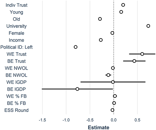
sjPlot::plot_model(m4)
Exercise 2: Longer panel data estimation with {plm}
Panel data gathers information about several individuals (cross-sectional units) over several periods. The panel is balanced if all units are observed in all periods; if some units are missing in some periods, the panel is unbalanced. A wide panel has the cross-sectional dimension (N) much larger than the longitudinal dimension (T); when the opposite is true, we have a long panel. Normally, the same units are observed in all periods; when this is not the case and each period samples mostly other units, the result is not a proper panel data, but pooled cross-sections model.
In the previous example the “panels” were fairly short. In this exercise, we use longer panel data to also demonstrate some additional functionalities in the plm package. The dataset is more typical of econometric data and originates from Hill et al.’s book “Principles of Econometrics”.
We can load the dataset directly from the book’s website website:
nls <- data_read("http://www.principlesofeconometrics.com/stata/nls_panel.dta")We can peek at the data to get a feel for the variables:
datawizard::data_peek(nls)| Data frame with 3580 rows and 18 variables | ||
|---|---|---|
| Variable | Type | Values |
| id | numeric | 1, 1, 1, 1, 1, 2, 2, 2, 2, 2, 3, 3, 3, 3, 3, ... |
| year | numeric | 82, 83, 85, 87, 88, 82, 83, 85, 87, 88, 82, ... |
| lwage | numeric | 1.80828905105591, 1.8634170293808, ... |
| hours | numeric | 38, 38, 38, 40, 40, 48, 43, 35, 42, 42, 48, ... |
| age | numeric | 30, 31, 33, 35, 37, 36, 37, 39, 41, 43, 35, ... |
| educ | numeric | 12, 12, 12, 12, 12, 17, 17, 17, 17, 17, 12, ... |
| collgrad | numeric | 0, 0, 0, 0, 0, 1, 1, 1, 1, 1, 0, 0, 0, 0, 0, ... |
| msp | numeric | 1, 1, 0, 0, 0, 1, 1, 1, 1, 1, 1, 1, 1, 1, 1, ... |
| nev_mar | numeric | 0, 0, 0, 0, 0, 0, 0, 0, 0, 0, 0, 0, 0, 0, 0, ... |
| not_smsa | numeric | 0, 0, 0, 0, 0, 0, 0, 0, 0, 0, 0, 0, 0, 0, 0, ... |
| c_city | numeric | 1, 1, 1, 1, 1, 0, 0, 0, 0, 0, 0, 0, 0, 0, 0, ... |
| south | numeric | 0, 0, 0, 0, 0, 0, 0, 0, 0, 0, 0, 0, 0, 0, 0, ... |
| black | numeric | 1, 1, 1, 1, 1, 0, 0, 0, 0, 0, 0, 0, 0, 0, 0, ... |
| union | numeric | 1, 1, 1, 1, 1, 0, 0, 0, 1, 1, 0, 1, 0, 0, 0, ... |
| exper | numeric | 7.66666698455811, 8.58333301544189, ... |
| exper2 | numeric | 58.7777709960938, 73.6736068725586, ... |
| tenure | numeric | 7.66666698455811, 8.58333301544189, ... |
| tenure2 | numeric | 58.7777709960938, 73.6736068725586, ... |
We can also check the first few and last few observations in a dataframe using the head() and tail() functions included in base-R. The gt package also has a nice function (gt_preview()) that can do the same more flexibly and output it as a single table:
## Complete the code field based on the code examples in the previous exerciseCheck the number of ids and years in the dataset:
## Complete the code field based on the code examples in the previous exerciseWe can also check the distribution of the variables:
## Complete the code field based on the code examples in the previous exercisePanel datsets can be organized in mainly two forms: the long form has a column for each variable and a row for each individual-period; the wide form has a column for each variable-period and a row for each individual. Most panel data methods require the long form, but many data sources provide one wide-form table for each variable; assembling the data from different sources into a long form data frame is often not a trivial matter.
The next code sequence creates a panel structure for the dataset using the function pdata.frame() of the plm package and displays a small part of this dataset:
nlspd <- pdata.frame(nls, index=c("id", "year"))The function pdim() extracts the dimensions of the panel data:
pdim(nlspd)Balanced Panel: n = 716, T = 5, N = 3580In the following, we will fit a series of models estimating wage as a function of education, experience (and a second-order polynomial for experience) and race (“black” vs. “white”), with the aim of demonstrating functions in the plm() package. We could also fit these models using the hierarchical modelling functions form previous examples and exercises.
Pooled model
A pooled model does not allow for intercept or slope differences among individuals. Such a model can be estimated with plm() using the specification pooling:
Check a summary of the results:
## Complete the code field based on the code examples in the previous exerciseFixed effects model
The fixed effects model takes into account individual differences, translated into different intercepts of the regression line for different individuals. Variables that change little or not at all over time, such as some individual characteristics should not be included in a fixed effects model because they produce collinearity with the fixed effects.
To estimate a fixed effects with plm, we can use the option model=“within”, and dummy variables for individuals are created automatically in the background and included in the model:
Check a summary of the results:
## Complete the code field based on the code examples in the previous exerciseWe can see in the results that the “race” variable was excluded from the model because it does not vary over time (it stays constant “within” an individual). This is one major limitation of so-called fixed effects (“within”) models.
The within method is equivalent to including the individual “indicators” in the model.
Random effects
The random effects model elaborates on the fixed effects model by recognizing that, since the individuals in the panel are randomly selected, their characteristics, measured by the intercept \(\beta_{1i}\) should also be random. Random effects estimators are reliable under the assumption that individual characteristics (heterogeneity) are exogenous, that is, they are independent with respect to the regressors in the random effects equation. We have already fit random effects models using the lme4 packages previously.
In plm, the same function we used for fixed effects can be used for random effects, but setting the argument model= to ‘random’ and selecting the random.method as one out of four possibilities: “swar” (default), “amemiya”, “walhus”, or “nerlove”:
Check a summary of the results:
## Complete the code field based on the code examples in the previous exerciseTabulating all the models:
We can now collate the models into a summary table to compare them more closely:
modelsummary::modelsummary(list(wage.pooled,
                                wage.within,
wage.random))| (1) | (2) | (3) | |
|---|---|---|---|
| (Intercept) | 0.427 | 0.476 | |
| (0.057) | (0.081) | ||
| educ | 0.075 | 0.075 | |
| (0.003) | (0.005) | ||
| exper | 0.063 | 0.055 | 0.056 |
| (0.008) | (0.006) | (0.006) | |
| I(exper^2) | -0.001 | -0.001 | -0.001 |
| (0.000) | (0.000) | (0.000) | |
| black | -0.136 | -0.136 | |
| (0.015) | (0.030) | ||
| Num.Obs. | 3580 | 3580 | 3580 |
| R2 | 0.288 | 0.131 | 0.176 |
| R2 Adj. | 0.287 | -0.087 | 0.175 |
| AIC | 3467.1 | -2290.1 | -1488.2 |
| BIC | 3504.2 | -2271.6 | -1451.1 |
| RMSE | 0.39 | 0.18 | 0.20 |
Exercise 3
Conduct a similar analysis as in Exercise 2 above, but using hierarchical modelling functions such as the lmer() function we used in earlier examples and exercises. Add the results to the summary table produced at the end of the previous exercise and compare the results across the modelling options.
Exercise 3
Return to the models based on Österman (2021) Table 3 from the Week 5 lab and expand those models to also include the survey “round” variable (essround) as an additional level accounting for variation across rounds/time.
Include these new models in a summary table to contrast the results from the previous models and reflect on the differences.
References
Mitchell, Jeffrey. 2021. “Social Trust and Anti-Immigrant Attitudes in Europe: A Longitudinal Multi-Level Analysis.” Frontiers in Sociology 6.
Österman, Marcus. 2021. “Can We Trust Education for Fostering Trust? Quasi-experimental Evidence on the Effect of Education and Tracking on Social Trust.” Social Indicators Research 154(1):211–33. doi: 10.1007/s11205-020-02529-y.